Diwali Sales Data
Diwali Sales Data

- The Diwali Sales dataset, featured in the TidyTuesday project for the week of November 14, 2023, provides a comprehensive look at retail sales during the Diwali festival in India. It offers a detailed snapshot of consumer behavior during one of the most significant festive periods in India.
Key Business Questions
- Which age group spends the most during Diwali?
- How does expenditure vary across genders within each age group?
- What are the common occupations of individuals in the highest spending age group?
- Which states have the highest spending, and how does this vary by gender?
- How does marital status influence spending patterns across different states and genders?
Insights and Trends
-
Age Group Spending:
- The age group 26-35 spends the most during Diwali. This demographic is likely to have higher disposable income and a greater inclination towards festive shopping.
-
Gender-Based Expenditure:
- Within each age group, spending patterns vary significantly between genders. In general, females tend to spend more than males across all age groups.
-
Occupational Insights:
- For individuals aged 26-35, the predominant occupations are in IT, healthcare, aviation, and banking. This suggests that marketing strategies aimed at these professional groups could be advantageous.
-
State-Wise Spending:
- States such as Uttar Pradesh, Maharashtra, Karnataka, and Delhi rank among the highest in spending.
-
Marital Status Influence:
- Married individuals tend to spend more than unmarried ones. This trend is consistent across both genders.
Recommendations
-
Targeted Marketing Campaigns:
- Focus marketing efforts on the 26-35 age group, especially targeting professionals and business owners. Tailor campaigns to highlight products and offers that appeal to this demographic.
-
Gender-Specific Strategies:
- Develop gender-specific marketing strategies. For example, create campaigns that resonate with female consumers in high-spending states.
-
State-Specific Promotions:
- Implement state-specific promotions, particularly in states with high spending. Customize offers and discounts to cater to the preferences of consumers in these regions.
-
Enhanced Customer Engagement:
- Use insights from occupational data to engage with customers through personalized communication. Offer exclusive deals and loyalty programs for professionals.
diwali <- read.csv("Diwali Sales Data.csv")
glimpse(diwali)
## Rows: 11,251
## Columns: 15
## $ User_ID <int> 1002903, 1000732, 1001990, 1001425, 1000588, 1000588,…
## $ Cust_name <chr> "Sanskriti", "Kartik", "Bindu", "Sudevi", "Joni", "Jo…
## $ Product_ID <chr> "P00125942", "P00110942", "P00118542", "P00237842", "…
## $ Gender <chr> "F", "F", "F", "M", "M", "M", "F", "F", "M", "F", "M"…
## $ Age.Group <chr> "26-35", "26-35", "26-35", "0-17", "26-35", "26-35", …
## $ Age <int> 28, 35, 35, 16, 28, 28, 25, 61, 35, 26, 34, 20, 20, 2…
## $ Marital_Status <int> 0, 1, 1, 0, 1, 1, 1, 0, 0, 1, 0, 0, 1, 1, 1, 0, 1, 0,…
## $ State <chr> "Maharashtra", "Andhra\xa0Pradesh", "Uttar Pradesh", …
## $ Zone <chr> "Western", "Southern", "Central", "Southern", "Wester…
## $ Occupation <chr> "Healthcare", "Govt", "Automobile", "Construction", "…
## $ Product_Category <chr> "Auto", "Auto", "Auto", "Auto", "Auto", "Auto", "Auto…
## $ Orders <int> 1, 3, 3, 2, 2, 1, 4, 1, 2, 4, 1, 2, 2, 4, 3, 2, 3, 1,…
## $ Amount <dbl> 23952.00, 23934.00, 23924.00, 23912.00, 23877.00, 238…
## $ Status <lgl> NA, NA, NA, NA, NA, NA, NA, NA, NA, NA, NA, NA, NA, N…
## $ unnamed1 <lgl> NA, NA, NA, NA, NA, NA, NA, NA, NA, NA, NA, NA, NA, N…Data Cleaning
- Renaming Andhra\xa0Pradesh to Andhra Pradesh.
- Converting Marital_Status column values to a factor.
- This would help with clear color differentiation for 1 (as red) and 2 (as blue), instead of a color range of values between 0 and 1.
- Removing columns that contain only NA values.
- Getting rid of rows where there aren’t any values recorded for the Amount column.
diwali <- diwali |>
    mutate(State = recode(State, "Andhra\xa0Pradesh" = "Andhra Pradesh"), .keep = "all" ) |>
    mutate(Marital_Status = as.factor(Marital_Status)) |>
    select(-Status, -unnamed1) |>
    filter(!is.na(Amount))

glimpse(diwali)
## Rows: 11,239
## Columns: 13
## $ User_ID <int> 1002903, 1000732, 1001990, 1001425, 1000588, 1000588,…
## $ Cust_name <chr> "Sanskriti", "Kartik", "Bindu", "Sudevi", "Joni", "Jo…
## $ Product_ID <chr> "P00125942", "P00110942", "P00118542", "P00237842", "…
## $ Gender <chr> "F", "F", "F", "M", "M", "M", "F", "M", "F", "M", "F"…
## $ Age.Group <chr> "26-35", "26-35", "26-35", "0-17", "26-35", "26-35", …
## $ Age <int> 28, 35, 35, 16, 28, 28, 25, 35, 26, 34, 20, 20, 26, 2…
## $ Marital_Status <fct> 0, 1, 1, 0, 1, 1, 1, 0, 1, 0, 0, 1, 1, 0, 0, 1, 1, 1,…
## $ State <chr> "Maharashtra", "Andhra Pradesh", "Uttar Pradesh", "Ka…
## $ Zone <chr> "Western", "Southern", "Central", "Southern", "Wester…
## $ Occupation <chr> "Healthcare", "Govt", "Automobile", "Construction", "…
## $ Product_Category <chr> "Auto", "Auto", "Auto", "Auto", "Auto", "Auto", "Auto…
## $ Orders <int> 1, 3, 3, 2, 2, 1, 4, 2, 4, 1, 2, 2, 4, 2, 1, 1, 1, 4,…
## $ Amount <dbl> 23952.00, 23934.00, 23924.00, 23912.00, 23877.00, 238…What age group spent the most?
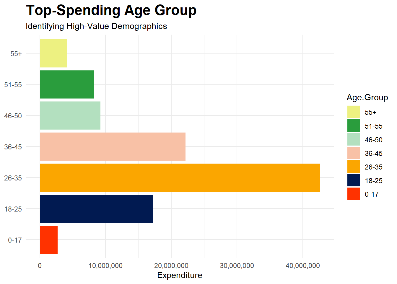
diwali |>
    select(Age.Group, Amount) |>
    arrange(Age.Group) |>
    group_by(Age.Group) |>
    summarise(Total_Amount = sum(Amount)) |>
    ggplot(aes(Age.Group, Total_Amount, fill = Age.Group)) +
    geom_col() +
    scale_fill_manual(values = col_theme) +
    labs(
        title = "Top-Spending Age Group",
        subtitle = "Identifying High-Value Demographics",
        x = NULL,
        y = "Expenditure"
            ) +
    theme(plot.title = element_text(size = 18, face = "bold")) +
    scale_y_continuous(labels = comma) +
    guides(fill = guide_legend(reverse = TRUE)) +
    coord_flip()
What is the expenditure across genders for each age group
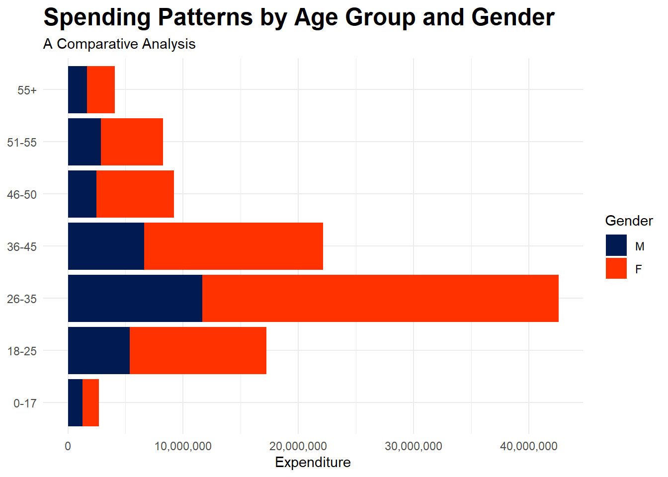
diwali |>
    select(Age.Group, Gender, Amount) |>
    arrange(Age.Group) |>
    group_by(Age.Group, Gender) |>
    summarise(Total_Amount = sum(Amount), .groups = "drop") |>
    ggplot(aes(Age.Group, Total_Amount, fill = Gender)) +
    geom_col() +
    scale_fill_manual(values = col_theme) +
    labs(
        title = "Spending Patterns by Age Group and Gender",
        subtitle = "A Comparative Analysis",
        x = NULL,
        y = "Expenditure"
            ) +
    theme(plot.title = element_text(size = 18, face = "bold")) +
    scale_y_continuous(labels = comma) +
    guides(fill = guide_legend(reverse = TRUE)) +
    coord_flip()
What are the occupations of people between 26-35
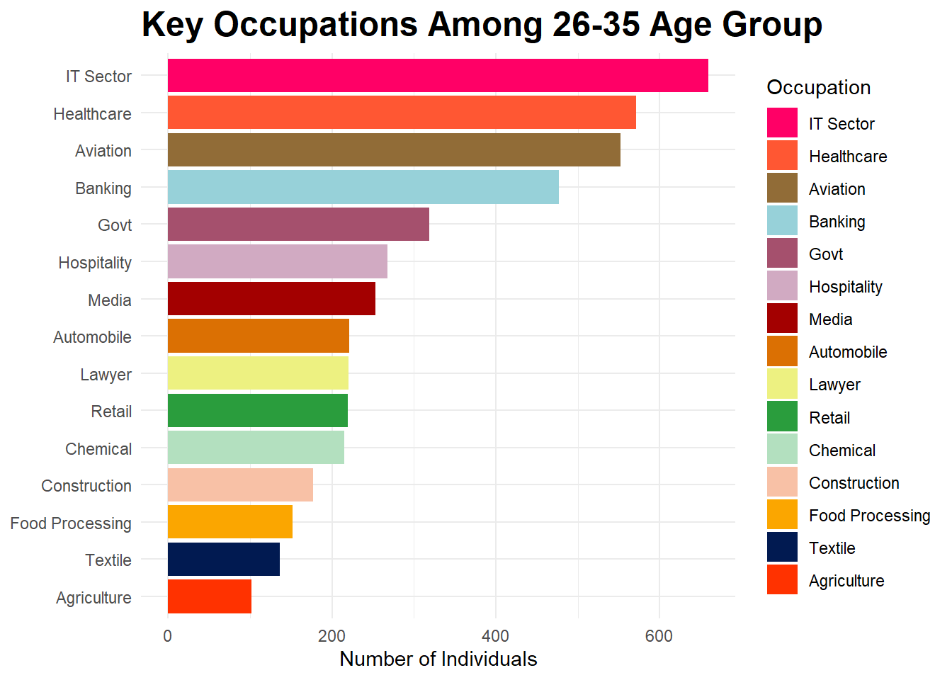
diwali |>
    select(Age.Group, Occupation) |>
    filter(Age.Group == "26-35") |>
    group_by(Occupation) |>
    summarise(Number_Of_Individuals = n()) |>
    mutate(Occupation = fct_reorder(Occupation, Number_Of_Individuals)) |>
    ggplot(aes(Occupation, Number_Of_Individuals, fill = Occupation)) +
    geom_col() +
    scale_fill_manual(values = col_theme) +
    labs(
        title = "Key Occupations Among 26-35 Age Group",
        x = NULL,
        y = "Number of Individuals"
            ) +
    theme(plot.title = element_text(size = 18, face = "bold")) +
    scale_y_continuous(labels = comma) +
    guides(fill = guide_legend(reverse = TRUE)) +
    coord_flip()
Which state spent the most (segregated by gender)?
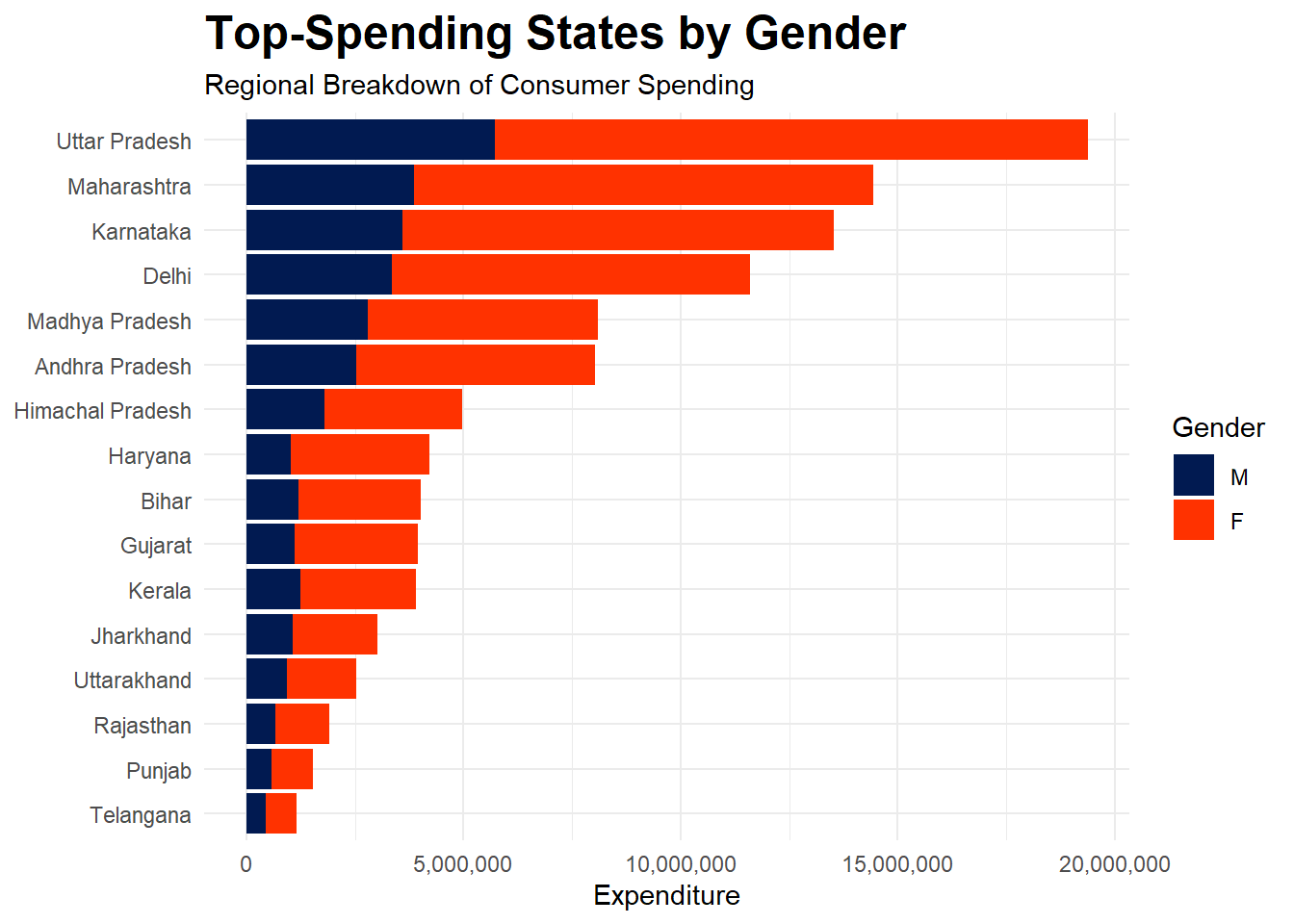
diwali |>
select(State, Amount, Gender) |>
group_by(State, Gender) |>
summarise(Total_Amount = sum(Amount), .groups = "drop") |>
mutate(State = fct_reorder(State, Total_Amount)) |>
ggplot(aes(State, Total_Amount, fill = Gender)) +
geom_col() +
scale_fill_manual(values = col_theme) +
labs(
    title = "Top-Spending States by Gender",
    subtitle = "Regional Breakdown of Consumer Spending",
    x = NULL,
    y = "Expenditure"
        ) +
theme(plot.title = element_text(size = 18, face = "bold")) +
scale_y_continuous(labels = comma) +
guides(fill = guide_legend(reverse = TRUE)) +
coord_flip()
Finding expenditure of females and males along with thier marital status
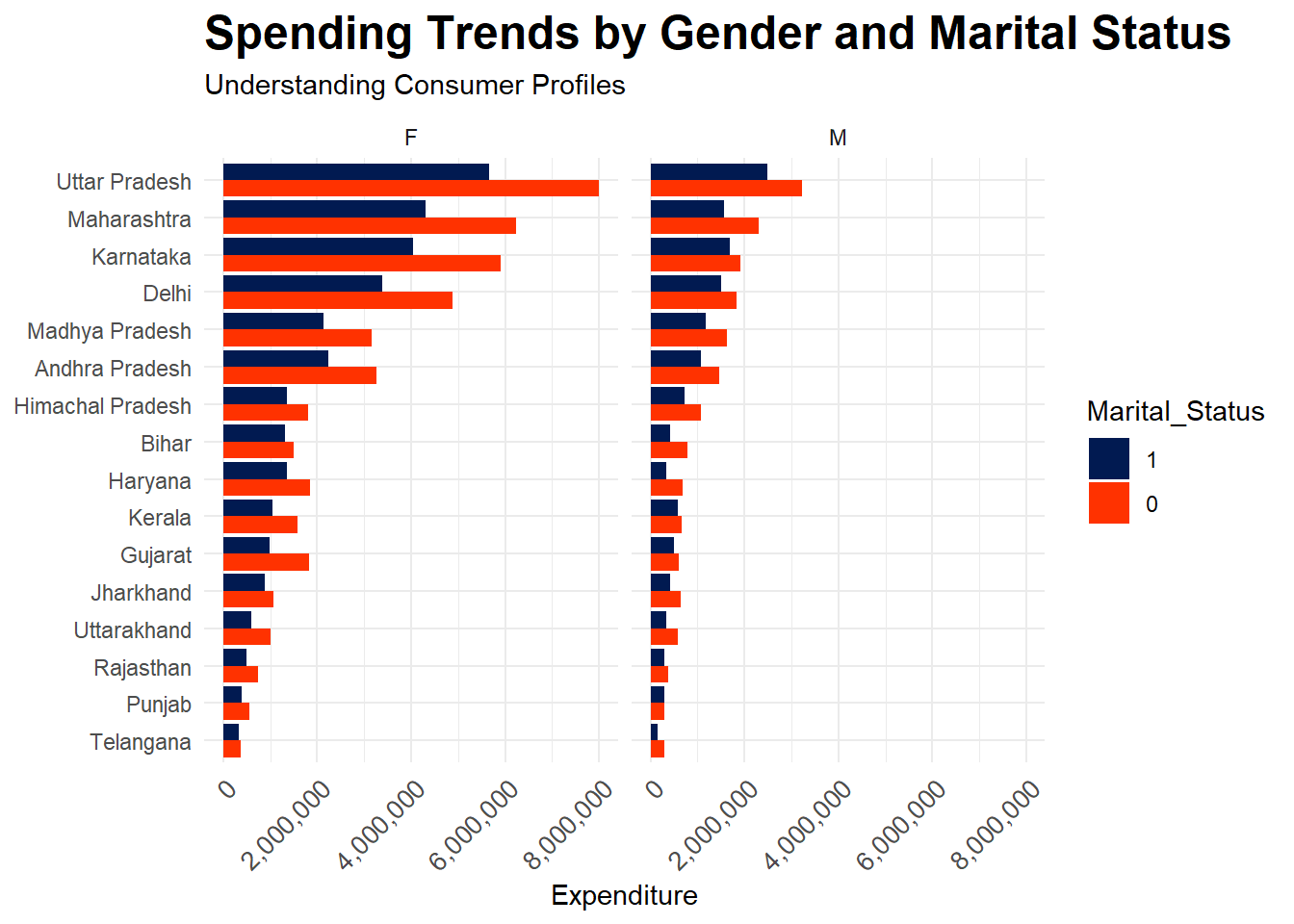
diwali |>
    select(State, Marital_Status, Gender, Amount) |>
    arrange(State, Gender) |>
    group_by(State, Gender, Marital_Status) |>
    summarise(Total_Amount = sum(Amount), .groups = "drop") |>
    mutate(State = fct_reorder(State, Total_Amount)) |>
    ggplot(aes(State, Total_Amount, fill = Marital_Status)) +
    geom_bar(stat = "identity", position = "dodge") +
    labs(title = "Comapring expenditures between married and unmarried individuals",
         subtitle = "Segregated by gender") +
    facet_wrap(~ Gender) +
    coord_flip() +
    theme(axis.text.x = element_text(angle = 45, hjust = 1, size = 10)) +
    scale_fill_manual(values = col_theme) +
    labs(
        title = "Spending Trends by Gender and Marital Status",
        subtitle = "Understanding Consumer Profiles",
        x = NULL,
        y = "Expenditure"
            ) +
    theme(plot.title = element_text(size = 18, face = "bold")) +
    guides(fill = guide_legend(reverse = TRUE)) +
    scale_y_continuous(labels = comma)
Last updated on